An Introduction to BayesHMM

Luis Damiano, Michael Weylandt, Brian Peterson

2019-01-03

BayesHMM is an R Package to run full Bayesian inference on Hidden Markov Models (HMM) using the probabilistic programming language Stan. By providing an intuitive, expressive yet flexible input interface, we enable researchers to profit the most out of the Bayesian workflow. We provide the user with an expressive interface to mix and match a wide array of options for the observation and latent models, including ample choices of densities, priors, and link functions whenever covariates are present. The software enables users to fit HMM with time-homogeneous transitions as well as time-varying transition probabilities. Priors can be set for every model parameter. Implemented inference algorithms include forward (filtering), forward-backwards (smoothing), Viterbi (most likely hidden path), prior predictive sampling, and posterior predictive sampling. Graphs, tables and other convenience methods for convergence diagnosis, goodness of fit, and data analysis are provided.

This vignette introduces the software and briefly reviews current capabilities. Although we walk the reader through most of the functionalities, we do not discuss function arguments, implementation details, and other details typically reviewed in the documentations. A list of future features may be found in the Roadmap wiki page.

NOTE: Our software is work in progress. We will review naming conventions as well as other design decisions at a later stage. Fully detailed documentation will be available at the time of release.

Introduction

Hidden Markov Models

Real-world processes produce observable outputs characterized as signals. These can be discrete or continuous in nature, be pure or contaminated with noise, come from a stationary or non stationary source, among many other variations. These signals are modelled to allow for both theoretical descriptions and practical applications. The model itself can be deterministic or stochastic, in which case the signal is well characterized as a parametric random process whose parameters can be estimated in a well-defined manner.

Autocorrelation, a key feature in most signals, can be modelled in countless forms. While certainly pertinent to this purpose, high-order Markov chains can prove inconvenient when the range of the correlation amongst the observations is long. A more parsimonious approach assumes that the observed sequence is a noisy observation of an underlying hidden process represented as a first-order Markov chain. In other terms, long-range dependencies between observations are mediated via latent variables. It is important to note that the Markov property is only assumed for the hidden states and not for the observations themselves.

Hidden Markov Models (HMM) involve two interconnected models. The state model consists of a discrete-time, discrete-state first-order Markov chain \(z_t \in \{1, \dots, K\}\) that transitions according to \(p(z_t | z_{t-1})\). In turns, the observation model is governed by \(p({\mathbf{y}}_t | z_t)\), where \({\mathbf{y}}_t \in {\mathbb{R}}^R\) are the observations, emissions or output. The corresponding joint distribution is

\[ p({\mathbf{z}}_{1:T}, {\mathbf{y}}_{1:T}) = p({\mathbf{z}}_{1:T}) p({\mathbf{y}}_{1:T} | {\mathbf{z}}_{1:T}) = \left[ p(z_1) \prod_{t=2}^{T}{p(z_t | z_{t-1})} \right] \left[ \prod_{t=1}^{T}{p({\mathbf{y}}_t | z_{t})} \right]. \]

The non-stochastic quantities of the model are the length of the observed sequence \(T\) and the number of hidden states \(K\). The observed sequence \({\mathbf{y}}_t\) is a stochastic known quantity. The parameters of the models are \({\mathbf{\theta}} = ({\mathbf{\pi}}, {\mathbf{\theta}}_t, {\mathbf{\theta}}_o)\), where \({\mathbf{\pi}}\) are the probabilities of the initial state distribution, \({\mathbf{\theta}}_t\) are the parameters of the transition model and \({\mathbf{\theta}}_o\) are the parameters of the state-conditional density function \(p({\mathbf{y}}_t | z_t)\). Their forms depend on the characteristics of the model specified by the user.

Observation model

The observation model is specified by the density \(p({\mathbf{y}}_t | z_{t})\). When the output is discrete, it commonly takes the form of an observation matrix

\[ p({\mathbf{y}}_t | z_t = k, {\mathbf{\theta}}) = \text{Categorical}({\mathbf{y}}_t | {\mathbf{\theta}}_k). \]

If the output is continuous, observations may follow for example a conditional Gaussian distribution

\[ p({\mathbf{y}}_t | z_t = k, {\mathbf{\theta}}) = \mathcal{N}({\mathbf{y}}_t | {\mathbf{\mu}}_k, {\mathbf{\Sigma}}_k). \]

Alternatively, time-varying covariates \({\mathbf{x}}_t \in {\mathbb{R}}^M\) may be used to drive the location parameter of the chosen density,

\[ p({\mathbf{y}}_t | {\mathbf{x}}_t, z_t = k, {\mathbf{\theta}}) = \mathcal{N}({\mathbf{y}}_t | {\mathbf{x}}_t {\mathbf{\beta}}^x_k, {\mathbf{\Sigma}}_k). \]

Transition model

In the most common case of time-homogeneous HMMs, state transitions are characterized by the \(K \times K\) sized transition matrix with simplex rows \({\mathbf{A}} = \{a_{ij}\}\) with \(a_{ij} = p(z_t = j | z_{t-1} = i)\). There are \(K \times (K-1)\) free parameters as the rows of the matrix must sum to one.

Alternatively, time-varying covariates \({\mathbf{u}}_t \in {\mathbb{R}}^P\) may be used to drive the location parameter of the chosen density, effectively allowing for time-varying transition probabilities. The model involves a multinomial regression whose parameters depend on the previous state taking the value \(i\). Using the softmax transform, for example,

\[ p(z_t | {\mathbf{u}}_{t}, z_{t-1} = i) = \text{softmax}({\mathbf{u}}_{t} {\mathbf{\beta}}^u_i). \]

Initial distribution model

Most frequently in applications, the initial distribution model is characterized by a \(K\) sized simplex \({\mathbf{\pi}}\) with initial probabilities \(\pi_{i} = p(z_1 = i)\). Alternatively, the first observation may be assigned to a state via a multinomial regression if relevant information is available in the form of a covariate vector \({\mathbf{v}} \in {\mathbb{R}}^Q\),

\[ p(z_1 | {\mathbf{v}}, {\mathbf{\theta}}) = \text{softmax}({\mathbf{v}} {\mathbf{\beta}}^v). \]

Inference

There are several quantities of interest that can be inferred via different algorithms. Our code contains the implementation of the most relevant methods for unsupervised data: forward, forward-backward and Viterbi decoding algorithms. We acknowledge the authors of the Stan Manual for the thorough illustrations and code snippets, some of which served as a starting point for our own code. As estimation is treated later, we assume that model parameters \({\mathbf{\theta}}\) are known.

Summary of the hidden quantities and their corresponding inference algorithm. \(\dagger\) Time complexity is reduced to \(O(KT)\) for inference on a left-to-right (upper triangular) transition matrix.

Name	Hidden Quantity	Availability at	Algorithm	Complexity
Filtering	\(p(z_t | {\mathbf{y}}_{1:t})\)	\(t\) (online)	Forward	\(O(K^2T)\)  \(O(KT)\dagger\)
Smoothing	\(p(z_t | {\mathbf{y}}_{1:T})\)	\(T\) (offline)	Forward-backward	\(O(K^2T)\)  \(O(KT)\dagger\)
Fixed lag smoothing	\(p(z_{t - \ell} | {\mathbf{y}}_{1:t})\), \(\ell \ge 1\)	\(t + \ell\) (lagged)	Forward-backward	\(O(K^2T)\)  \(O(KT)\dagger\)
State prediction	\(p(z_{t+h} | {\mathbf{y}}_{1:t})\), \(h\ge 1\)	\(t\)
Observation prediction	\(p(y_{t+h} | {\mathbf{y}}_{1:t})\), \(h\ge 1\)	\(t\)
MAP Estimation	\({\arg\!\max}_{{\mathbf{z}}_{1:T}} p({\mathbf{z}}_{1:T} | {\mathbf{y}}_{1:T})\)	\(T\)	Viterbi decoding	\(O(K^2T)\)
Log likelihood	\(p({\mathbf{y}}_{1:T})\)	\(T\)	Forward	\(O(K^2T)\)  \(O(KT)\dagger\)

Filtering

A filter infers the posterior distribution of the hidden states at a given step \(t\) based on all the information available up to that point \(p(z_t | {\mathbf{y}}_{1:t})\). It achieves better noise reduction than simply estimating the hidden state based on the current estimate \(p(z_t | {\mathbf{y}}_{t})\). The filtering process can be run online, or recursively, as new data streams in.

Filtered marginals can be computed recursively using the forward algorithm [@baum1967inequality]. Let \(\psi_t(j) = p({\mathbf{y}}_t | z_t = j)\) be the local evidence at step \(t\) and \(\Psi(i, j) = p(z_t = j | z_{t-1} = i)\) be the transition probability. First, the one-step-ahead predictive density is computed

\[ p(z_t = j | {\mathbf{y}}_{1:t-1}) = \sum_{i}{\Psi(i, j) p(z_{t-1} = i | {\mathbf{y}}_{1:t-1})}. \]

Acting as prior information, this quantity is updated with observed data at the step \(t\) using the Bayes rule,

\[\begin{align*} \label{eq:filtered-beliefstate} \alpha_t(j) & \triangleq p(z_t = j | \mat{y}_{1:t}) \\ &= p(z_t = j | \mat{y}_{t}, \mat{y}_{1:t-1}) \\ &= Z_t^{-1} \psi_t(j) p(z_t = j | \mat{y}_{1:t-1}) \\ \end{align*}\]

where the normalization constant is given by

\[ Z_t \triangleq p({\mathbf{y}}_t | {\mathbf{y}}_{1:t-1}) = \sum_{l=1}^{K}{p({\mathbf{y}}_{t} | z_t = l) p(z_t = l | {\mathbf{y}}_{1:t-1})} = \sum_{l=1}^{K}{\psi_t(l) p(z_t = l | {\mathbf{y}}_{1:t-1})}. \]

This predict-update cycle results in the filtered belief states at step \(t\). As this algorithm only requires the evaluation of the quantities \(\psi_t(j)\) for each value of \(z_t\) for every \(t\) and fixed \({\mathbf{y}}_t\), the posterior distribution of the latent states is independent of the form of the observation density or indeed of whether the observed variables are continuous or discrete [@jordan2003introduction]. In other words, \(\alpha_t(j)\) does not depend on the complete form of the density function \(p({\mathbf{y}} | {\mathbf{z}})\) but only on the point values \(p({\mathbf{y}}_t | z_t = j)\) for every \({\mathbf{y}}_t\) and \(z_t\).

Let \({\mathbf{\alpha}}_t\) be a \(K\)-sized vector with the filtered belief states at step \(t\), \({\mathbf{\psi}}_t(j)\) be the \(K\)-sized vector of local evidence at step \(t\), \({\mathbf{\Psi}}\) be the transition matrix and \({\mathbf{u}} \odot {\mathbf{v}}\) be the Hadamard product, representing element-wise vector multiplication. Then, the Bayesian updating procedure can be expressed in matrix notation as

\[ {\mathbf{\alpha}}_t \propto {\mathbf{\psi}}_t \odot ({\mathbf{\Psi}}^T {\mathbf{\alpha}}_{t-1}). \]

In addition to computing the hidden states, the algorithm yields the log likelihood

\[ {\mathcal{L}}= \log p({\mathbf{y}}_{1:T} | {\mathbf{\theta}}) = \sum_{t=1}^{T}{\log p({\mathbf{y}}_{t} | {\mathbf{y}}_{1:t-1})} = \sum_{t=1}^{T}{\log Z_t}. \]

The time complexity of the algorithm is \(O(K^2T)\): there are \(K \times K\) iterations within each of the \(T\) iterations of the outer loop. Brute-forcing through all possible hidden states \(K^T\) would prove prohibitive for realistic problems as time complexity increases exponentially with sequence length \(O(K^TT)\).

Smoothing

A smoother infers the posterior distribution of the hidden states at a given state based on all the observations or evidence \(p(z_t | {\mathbf{y}}_{1:T})\). Although noise and uncertainty are significantly reduced as a result of conditioning on past and future data, the smoothing process can only be run offline.

Inference can be done by means of the forward-backward algorithm, which also plays an important role in the Baum-Welch algorithm for learning model parameters [@baum1967inequality; @baum1970maximization]. Let \(\gamma_t(j)\) be the desired smoothed posterior marginal,

\[ \gamma_t(j) \triangleq p(z_t = j | {\mathbf{y}}_{1:T}), \]

\(\alpha_t(j)\) be the filtered belief state at the step \(t\) as defined previously, and \(\beta_t(j)\) be the conditional likelihood of future evidence given that the hidden state at step \(t\) is \(j\),

\[ \beta_t(j) \triangleq p({\mathbf{y}}_{t+1:T} | z_t = j). \]

Then, the chain of smoothed marginals can be segregated into the past and the future components by conditioning on the belief state \(z_t\),

\[ \gamma_t(j) = \frac{\alpha_t(j) \beta_t(j)}{p({\mathbf{y}}_{1:T})} \propto \alpha_t(j) \beta_t(j). \]

The future component can be computed recursively from right to left:

\[\begin{align*} \beta_{t-1}(i) &= p(\mat{y}_{t:T} | z_{t-1} = i) \\ &= \sum_{j=1}^{K}{p(z_t =j, \mat{y}_{t}, \mat{y}_{t+1:T} | z_{t-1} = i)} \\ &= \sum_{j=1}^{K}{p(\mat{y}_{t+1:T} | z_t = j)p(z_t = j, \mat{y}_{t} | z_{t-1} = i)} \\ &= \sum_{j=1}^{K}{p(\mat{y}_{t+1:T} | z_t = j)p(\mat{y}_t | z_t = j)p(z_t = j | z_{t-1} = i)} \\ &= \sum_{j=1}^{K}{\beta_t(j) \psi_t(j) \Psi(i, j)} \end{align*}\]

Let \({\mathbf{\beta}}_t\) be a \(K\)-sized vector with the conditional likelihood of future evidence given the hidden state at step \(t\). Then, the backward procedure can be expressed in matrix notation as

\[ {\mathbf{\beta}}_{t-1} \propto {\mathbf{\Psi}} ({\mathbf{\psi}}_t \odot {\mathbf{\beta}}_{t}). \]

At the last step, the base case is given by \[ \beta_{T}(i) = p({\mathbf{y}}_{T+1:T} | z_{T} = i) = p(\varnothing | z_t = i) = 1. \]

Intuitively, the forward-backward algorithm passes information from left to right and then from right to left, combining them at each node. A straightforward implementation of the algorithm runs in \(O(K^2 T)\) time because of the \(K \times K\) matrix multiplication at each step. Nonetheless the frequent description as two subsequent passes, these procedures are not inherently sequential and share no information. As a result, they could be implemented in parallel.

There is a significant reduction if the transition matrix is sparse. Inference for a left-to-right (upper triangular) transition matrix, a model where the state index increases or stays the same as time passes, runs in \(O(TK)\) time [@bakis1976continuous;@jelinek1976continuous]. Additional assumptions about the form of the transition matrix may ease complexity further, for example decreasing the time to \(O(TK\log K)\) if \(\psi(i, j) \propto \exp(-\sigma^2 |{\mathbf{z}}_i - {\mathbf{z}}_j|)\). Finally, ad-hoc data pre-processing strategies may help control complexity, for example by pruning nodes with low conditional probability of occurrence.

The forward-backward algorithm was designed to exploit via recursion the conditional independencies in the HMM. First, the posterior marginal probability of the latent states at a given time step is broken down into two quantities: the past and the future components. Second, taking advantage of the Markov properties, each of the two are further broken down into simpler pieces via conditioning and marginalizing, thus creating an efficient predict-update cycle.

This strategy makes otherwise unfeasible calculations possible. Consider for example a time series with \(T = 100\) observations and \(K = 5\) hidden states. Summing the joint probability over all possible state sequences would involve \(2 \times 100 \times 5^{100} \approx 10^{72}\) computations, while the forward and backward passes only take \(3,000\) each. Moreover, one pass may be avoided depending on the goal of the data analysis. Summing the forward probabilities at the last time step is enough to compute the likelihood, and the backwards recursion would be only needed if the posterior probabilities of the states were also required.

MAP: Viterbi

It is also of interest to compute the most probable state sequence or path,

\[ {\mathbf{z}}^* = {\arg\!\max}_{{\mathbf{z}}_{1:T}} p({\mathbf{z}}_{1:T} | {\mathbf{y}}_{1:T}). \]

The jointly most probable sequence of states can be inferred via maximum a posteriori (MAP) estimation. Note that the jointly most probable sequence is not necessarily the same as the sequence of marginally most probable states given by the maximizer of the posterior marginals (MPM),

\[ {\mathbf{\hat{z}}} = ({\arg\!\max}_{z_1} p(z_1 | {\mathbf{y}}_{1:T}), \ \dots, \ {\arg\!\max}_{z_T} p(z_T | {\mathbf{y}}_{1:T})), \]

which maximizes the expected number of correct individual states.

The MAP estimate is always globally consistent: while locally a state may be most probable at a given step, the Viterbi or max-sum algorithm decodes the most likely single plausible path [@viterbi1967error]. Furthermore, the MPM sequence may have zero joint probability if it includes two successive states that, while being individually the most probable, are connected in the transition matrix by a zero. On the other hand, MPM may be considered more robust since the state at each step is estimated by averaging over its neighbors rather than conditioning on a specific value of them.

The Viterbi applies the max-sum algorithm in a forward fashion plus a traceback procedure to recover the most probable path. In simple terms, once the most probable state \(z_t\) is estimated, the procedure conditions the previous states on it. Let \(\delta_t(j)\) be the probability of arriving to the state \(j\) at step \(t\) given the most probable path was taken,

\[ \delta_t(j) \triangleq \max_{z_1, \dots, z_{t-1}} p({\mathbf{z}}_{1:t-1}, z_t = j | {\mathbf{y}}_{1:t}). \]

The most probable path to state \(j\) at step \(t\) consists of the most probable path to some other state \(i\) at point \(t-1\), followed by a transition from \(i\) to \(j\),

\[ \delta_t(j) = \max_{i} \delta_{t-1}(i) \ \psi(i, j) \ \psi_t(j). \]

Additionally, the most likely previous state on the most probable path to \(j\) at step \(t\) is given by \[ a_t(j) = {\arg\!\max}_{i} \delta_{t-1}(i) \ \psi(i, j) \ \psi_t(j). \]

By initializing with \(\delta_1 = \pi_j \phi_1(j)\) and terminating with the most probable final state \(z_T^* = {\arg\!\max}_{i} \delta_T(i)\), the most probable sequence of states is estimated using the traceback,

\[ z_t^* = a_{t+1}(z_{t+1}^*). \]

It is advisable to work in the log domain to avoid numerical underflow,

\[ \delta_t(j) \triangleq \max_{{\mathbf{z}}_{1:t-1}} \log p({\mathbf{z}}_{1:t-1}, z_t = j | {\mathbf{y}}_{1:t}) = \max_{i} \log \delta_{t-1}(i) + \log \psi(i, j) + \log \psi_t(j). \]

As with the backward-forward algorithm, the time complexity of Viterbi is \(O(K^2T)\) and the space complexity is \(O(KT)\). If the transition matrix has the form \(\psi(i, j) \propto \exp(-\sigma^2 ||{\mathbf{z}}_i - {\mathbf{z}}_j||^2)\), implementation runs in \(O(TK)\) time.

Parameter estimation

The model likelihood can be derived from the definition of the quantity \(\gamma_t(j)\): given that its sum over all possible values of the latent variable must equal one, the log likelihood at time index \(t\) becomes

\[ {\mathcal{L}}_t = \sum_{i = 1}^{K}{\alpha_t(i) \beta_{t}(i)}. \]

The last step \(T\) has two convenient characteristics. First, the recurrent nature of the forward probability implies that the last iteration retains the information of all the intermediate state probabilities. Second, the base case for the backwards quantity is \(\beta_{T}(i) = 1\). Consequently, the log likelihood reduces to

\[ {\mathcal{L}}_T \propto \sum_{i = 1}^{K}{\alpha_T(i)}. \]

Naming convention

Documentation and software adopts the following naming convention. Minor modifications may be found due to syntax restrictions in R or Stan. Time suffix _t is optional.

Constants
R	Observation dimension
K	Number of hidden states
M	Number of covariates for the observation model
P	Number of covariates for the transition model
Q	Number of covariates for the initial model
Covariates
x_t	Time-varying covariates for the observation model
u_t	Time-varying covariates for the transition model
v	Covariates for the initial model
Known-stochastic quantities
y_t	Observation vector
Model parameters
*_kr	Ex. mu_11 or sigma_11 (suffixes k and r are optional)
A	Transition model parameters (if no covariates)
pi	Initial distribution parameters (if no covariates)
xBeta	Regression parameters for the observation model
uBeta	Regression parameters for the transition model
vBeta	Regression parameters for the initial model
Estimated quantities
z_t	Hidden state
alpha_t Filtered probability
gamma_t Smoothed probability
zstar	Viterbi
(Prior/Posterior) predictive quantities
yPred	Sample of observations drawn from the predictive density
zPred	Sample of latent path drawn from the predictive density

Using BayesHMM

The typical data analysis workflow includes the following steps: (1) specify, (2) validate, (3) simulate, (4) fit, (5) diagnose, (6) visualize, (7) compare. All steps except for 5 and 7 are implemented as of today.

You may install the lastest version of our software from GitHub. Please note that BayesHMM requires rstan (>= 2.17), the R interface for the probabilistic programming language Stan.

#> Loading required package: Rcpp
#> Hola! BayesHHM v0.0.1 here o/

devtools::install_github("luisdamiano/BayesHMM", ref = "master")
library(BayesHMM)

1. Specify

A HMM may be specified by calling the hmm function:

hmm(
  K = 3, R = 2,
  observation = {...}
  initial     = {...}
  transition  = {...}
  name = "Model name"
)

where \(K\) is the number of hidden states and \(R\) is the number of dimensions in the observation variable.

The observation, initial, and transition fields rely on S3 objects called Density to specify density form, parameter priors, and fixed values for parameters. User may specify bounds in the parameter space as well as truncation in prior densities. For example:

• Gaussian(mu = 0, sigma = 1) specifies a Gaussian density with fixed parameters.
• Gaussian(mu = Gaussian(0, 10), sigma = Cauchy(0, 10, bounds = list(0, NA))) specifies a Gaussian density with a Gaussian prior on the location parameter and a Cauchy prior on the scale parameter, which is bounded on \([0, \infty)\).

Currently available densities are listed below:

• Observation model:
  • Univariate: Bernoulli, Beta, Binomial, Categorical, Cauchy, Dirichlet, Gaussian, Multinomial, Negative Binomial (traditional and location parameterizations), Poisson, Student.
  • Multivariate: Multivariate Gaussian (traditional, Cholesky decomposition of covariance matrix, and Cholesky decomposition of correlation matrix parameterizations), Multivariate Student.
  • Regressions: Bernoulli regression with logit link, Binomial regression (logit and probit links), Softmax regression, Gaussian regression.
  • Prior-only density: LKJ, Wishart.
• Transition model: Dirichlet, Softmax regression.
• Initial model: Dirichlet, Softmax regression.

Observation model

Internally, a specification stores either \(K\) multivariate densities (i.e. one multivariate density for state) or \(K \times R\) univariate densities (i.e. one univariate density for each dimension in the observation variable and each state). As shown in the next table, densities are recycled to simplify user-input code.

R	User input	Density	Action
1	1	UnivariateDensity	repeat_K
1	K	UnivariateDensity	repeat_none
>1	1	MultivariateDensity	repeat_K
>1	1	UnivariateDensity	repeat_KxR
>1	K	MultivariateDensity	repeat_none
>1	K	UnivariateDensity	repeat_R
>1	R	UnivariateDensity	repeat_K
>1	KxR	UnivariateDensity	repeat_none

For a univariate model (\(R = 1\)):

• User enters one univariate density: specify the same density in each hidden state variable.
• User enters \(K\) univariate density: specify one different density in each hidden state (ex. Gaussian in one state and Student in the other).

This system is flexible enough to let the user specify different densities and priors for each state. The following example demonstrates a (rather unrealistic) model where states are a priori believed to have negative, near zero, and positive location parameters.

mySpec <- hmm(
  K = 3, R = 1,
  observation =
    Gaussian(mu = -10, sigma = 10) +
    Gaussian(mu =   0, sigma = 10) +
    Gaussian(mu =  10, sigma = 10),
  initial     = Dirichlet(alpha = ImproperUniform()),
  transition  = Dirichlet(alpha = ImproperUniform()),
  name = "Univariate Gaussian"
)

For a multivariate model (\(R > 1\)):

• User enters one univariate density: same density for each dimension of the observation variable in all states (i.e. same density and priors for the R variables in the K latent states).
• User enters one multivariate density: same density for the observation vector in all hidden states.
• User enters \(K\) univariate density: each dimension of the observation variable has the same specification within a each state.
• User enters \(K\) multivariate density: specify a multivariate density for the observation vector for each state.
• User enters \(R\) univariate density: specify one density for each element of the observation vector, which is the same across state.
• User enters \(R \times K\) univariate density: specify density for each element of the observation vector in each state. Order is \(k_1 r_1, \dots, k_1, r_R, k_2r_1, \dots, k_2r_R, \dots, k_Kr_1, \dots, k_K,r_R\).
• When \(K = R\), \(K\) prevails.

Transition model

The user may enter a Density S3 object such as a Dirichlet, or a LinkDensity S3 object (inherits from Density) such as TransitionSoftmax(). The latter allows to specify priors for the transition regression parameter vector. For example, the following example sets regularizing priors near zero on the regression coefficients (because softmax coefficients are location invariant, we use priors to better inform the model). Note that this model is hard to identify, although we achieved satisfactory results optimizing the posterior density (i.e. maximum a posterior estimates).

mySpec <- hmm(
  K = 2, R = 1,
  observation = Gaussian(
    mu    = Gaussian(0, 10),
    sigma = Student(mu = 0, sigma = 10, nu = 1, bounds = list(0, NULL))
  ),
  initial     = ImproperUniform(),
  transition  = TransitionSoftmax(
    uBeta = Gaussian(0, 5)
  ),
  name = "TVHMM Softmax Univariate Gaussian"
)

Internally, a specification stores either \(K\) multivariate densities (i.e. one multivariate density for each row in the transition matrix) or \(K \times K\) univariate densities (i.e. one univariate density for each element in the transition matrix). Densities are recycled accordingly.

User-input	Density	Action
1	UnivariateDensity	repeat_KxK
1	MultivariateDensity	repeat_K
1	LinkDensity	nothing
K	UnivariateDensity	repeat_K
K	MultivariateDensity	repeat_none_multivariate
KxK	UnivariateDensity	repeat_none_univariate

NOTE: As of the time of this writing, fixed values for transition parameters have not been implemented yet.

Initial model

Internally, a specification stores either one multivariate densities for the whole initial probability vector, or \(K\) univariate densities for each element of said vector. Densities are recycled accordingly.

User-input	Density	Action
1	UnivariateDensity	repeat_K
1	MultivariateDensity	repeat_none_multivariate
1	LinkDensity	repeat_none_multivariate
K	UnivariateDensity	repeat_none_univariate

mySpec <- hmm(
  K = 2, R = 1,
  observation = Gaussian(
    mu    = Gaussian(0, 10),
    sigma = Student(mu = 0, sigma = 10, nu = 1, bounds = list(0, NULL))
  ),
  initial     = InitialSoftmax(
    vBeta = Gaussian(0, 5)
  ),
  transition  = Dirichlet(alpha = ImproperUniform()),
  name = "Univariate Gaussian with covariates for initial model"
)

Examples

Many possible configurations are shown in the Appendix .

2. Validate

Bayesian Software Validation allows users to test software accuracy [CITE]. We provide a one-liner to run a validation protocol based on the prior predictive density. Iterations are run in parallel using foreach and doParallel.

Validation protocol inspired by Simulation Based Calibration (cite)

• Compile the prior predictive model (i.e. no likelihood statement in the Stan code).
• Draw \(N\) samples of the parameter vector \(\theta\) and the observation vector \({\mathbf{y}}_t\) from prior predictive density.
• Compile the posterior predictive model (i.e. Stan code includes both prior density and likelihood statement).
• For all \(n \in 1, \dots, N\):
  • Feed \({\mathbf{y}}_t^{(n)}\) to the full model.
  • Draw one posterior sample of the observation variable \({\mathbf{y_t}}^{(n)}_{\text{new}}\).
  • Collect Hamiltonian Monte Carlo diagnostics: number of divergences, number of times max tree depth is reached, maximum leapfrogs, warm up and sample times.
  • Collect posterior sampling diagnostics: posterior summary measures (mean, sd, quantiles), comparison against the true value (rank), MCMC convergence measures (Monte Carlo SE, ESS, R Hat).
  • Collect posterior predictive diagnostics: observation ranks, Kolmogorov-Smirnov statistic for observed sample vs posterior predictive samples.
  • Other: we expect to enrich the protocol with more relevant quantities in future iterations.

There is no such a thing as an universal, automatic way to validate models. The software computes and summarizes different diagnostic measures and provides the user with high-level tools to assess calibration (including printouts, tables, and plots). Because the user may want to single out and inspect one of the iterations, in future versions it will be able to recover (or reproduce) the full posterior sample drawn in the \(n\)-th iteration.

In the following example, we specify a HMM and validate its calibration.

  mySpec <- hmm(
    K = 3, R = 2,
    observation =
      Gaussian(mu = Gaussian(mu = -10, sigma = 1), sigma = 1) +
      Gaussian(mu = Gaussian(mu =   0, sigma = 1), sigma = 1) +
      Gaussian(mu = Gaussian(mu =  10, sigma = 1), sigma = 1),
    initial     = Dirichlet(alpha = c(0.5, 0.5, 0.5)),
    transition  =
      Dirichlet(alpha = c(1.0, 0.2, 0.2)) +
      Dirichlet(alpha = c(0.2, 1.0, 0.2)) +
      Dirichlet(alpha = c(0.2, 0.2, 1.0)),
    name = "Dummy Model"
  )

  val <- validate_calibration(mySpec, N = 2, T = 100, iter = 500, seed = 9000)
#> hash mismatch so recompiling; make sure Stan code ends with a blank line
#> hash mismatch so recompiling; make sure Stan code ends with a blank line

The function returns a named list with two elements, chains and parameters, which are data frames storing the aforementioned summary quantities.

knitr::kable(
  head(val$chains), 
  digits = 2, caption = "Chains diagnostics"
)

Chains diagnostics

model	chain	divergences	maxTreeDepth	maxNLeapfrog	warmup	sample	r1.y25Rank	r1.yMedRank	r1.y75Rank	r1.yMeanRank	r1.ksMean	r1.ksMedian	r2.y25Rank	r2.yMedRank	r2.y75Rank	r2.yMeanRank	r2.ksMean	r2.ksMedian	seed	n
Dummy Model	1	33	0	25	0.76	0.52	0.12	0.61	0.82	0.35	0.29	0.30	0.90	0.80	0.65	0.67	0.22	0.21	9000	1
Dummy Model	2	0	0	15	0.81	0.55	0.02	0.14	0.74	0.17	0.34	0.35	0.83	0.80	0.57	0.62	0.23	0.22	9000	1
Dummy Model	3	0	0	15	0.84	0.52	0.01	0.17	0.41	0.11	0.37	0.37	0.80	0.76	0.70	0.65	0.22	0.22	9000	1
Dummy Model	4	0	0	31	0.98	0.54	0.02	0.03	0.45	0.00	0.34	0.34	0.79	0.78	0.59	0.60	0.23	0.22	9000	1
Dummy Model	1	0	0	31	1.23	0.54	0.05	0.02	0.61	0.03	0.50	0.53	0.00	0.13	0.68	0.48	0.23	0.22	9000	2
Dummy Model	2	0	0	15	1.11	0.62	0.02	0.00	0.24	0.01	0.50	0.52	0.00	0.09	0.82	0.53	0.23	0.22	9000	2

knitr::kable(
  head(val$parameters), 
  digits = 2, caption = "Parameters diagnostics"
)

Parameters diagnostics

model	chain	parameter	mean	se_mean	sd	X2.5.	X25.	X50.	X75.	X97.5.	n_eff	Rhat	true	rank	n
Dummy Model	1	mu11	-10.10	0.10	1.14	-12.15	-10.96	-10.04	-9.26	-8.13	125.00	1.01	-11.47	0.10	1
Dummy Model	1	mu12	-10.64	0.01	0.09	-10.84	-10.68	-10.64	-10.58	-10.47	125.00	0.99	-9.91	1.00	1
Dummy Model	1	mu21	-0.03	0.10	1.01	-1.87	-0.77	-0.12	0.70	2.00	92.91	0.99	-0.46	0.34	1
Dummy Model	1	mu22	9.74	0.01	0.13	9.47	9.67	9.75	9.81	9.96	125.00	0.99	0.75	0.00	1
Dummy Model	1	mu31	9.91	0.12	0.95	8.23	9.28	9.72	10.58	11.98	62.18	1.00	10.48	0.74	1
Dummy Model	1	mu32	0.57	0.01	0.15	0.28	0.47	0.58	0.68	0.85	125.00	1.00	9.60	1.00	1

plot(
  val$parameters$Rhat, 
  type = "h", ylim = c(0.9, 1.15),
  ylab = expression(hat(R)),
  xlab = "Validation run (n)"
)
abline(h = 1.1)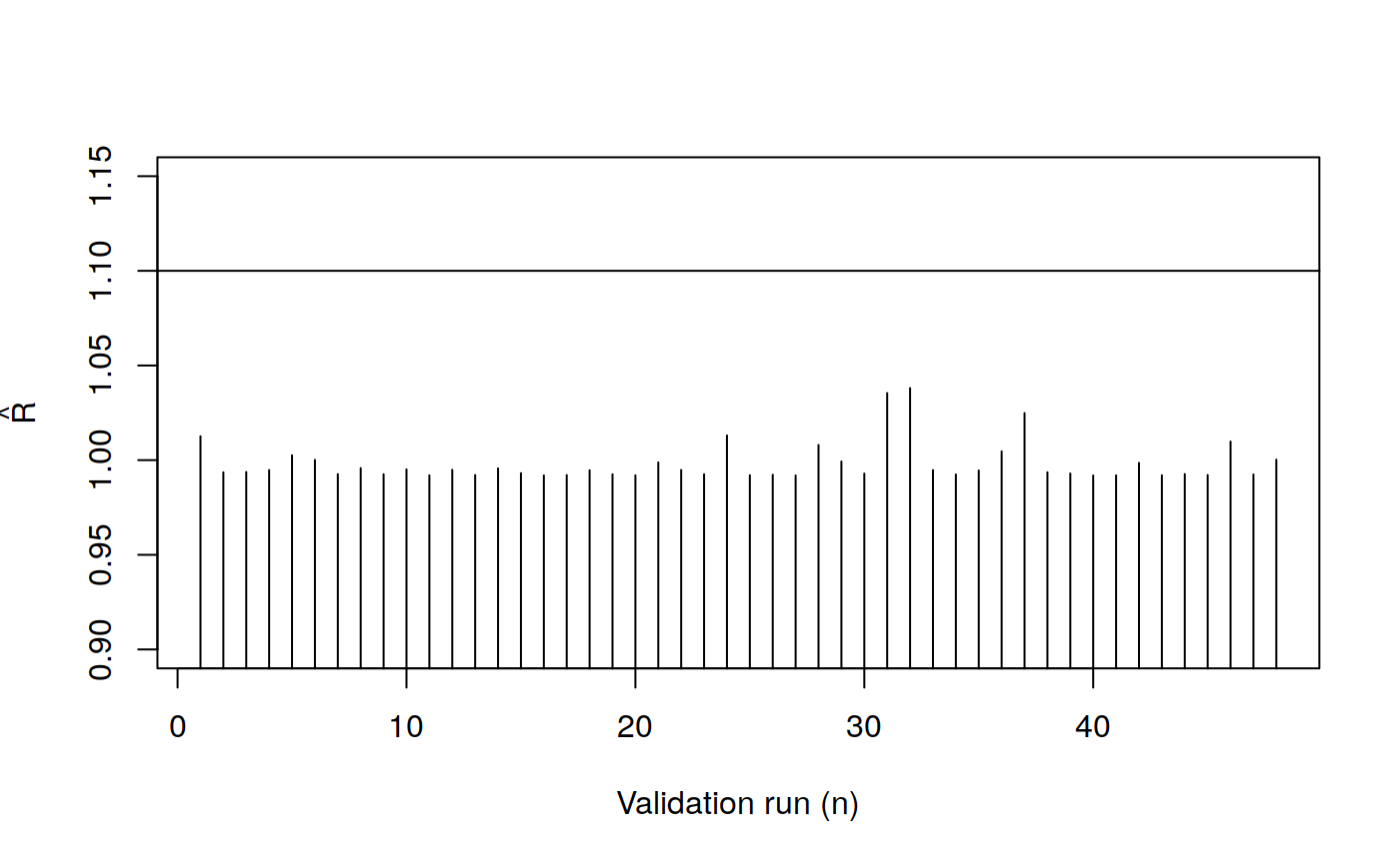

3. Simulate & Fit

Once specified, the user may:

• Call sim() to simulate \(N\) datasets containing the observation variables \({\mathbf{y}}\) and the hidden paths \(z\).
• Call compile() to compile the underlying Stan model. The returned object may be later used for either sampling (MCMC) or optimization (MAP).
  • Call sampling() to draw posterior samples from a compiled model effectively allowing for full Bayesian inference via MCMC.
  • Call optimizing() to maximize the joint posterior density and obtain a point estimate.
• Call fit() to compile and sample in one step.

After fitting, the underlying Stan code may be inspected by calling browse_model, which opens the Stan file in the editor. None that this function is only for reading purposes: changes in the Stan code will not affect the specification object.

3.1. Fully Bayesian Inferencia via MCMC

Because sampling() and fit() return a stanfit S4 object, the posterior samples are compatible out of box with the rstan ecosystem [TRY AND LIST SOME SUCH AS bayesplot].

3.2. Maximum a Posteriori estimates via posterior optimization

optimizing is able to run several initialization of the optimization algorithm in parallel. The user may decide to keep = "all" runs, or just keep = "best". If the former, extract_grid returns a summary of the different runs and extract_best retrieves the one with highest posterior log likelihood. If no run achieves convergence, a warning message is prompt to the console.

mySpec <- hmm(
  K = 3, R = 1,
  observation =
    Gaussian(mu = Gaussian(mu = -10, sigma = 1), sigma = 1) +
    Gaussian(mu = Gaussian(mu =   0, sigma = 1), sigma = 1) +
    Gaussian(mu = Gaussian(mu =  10, sigma = 1), sigma = 1),
  initial     = Dirichlet(alpha = c(0.5, 0.5, 0.5)),
  transition  = Dirichlet(alpha = c(0.5, 0.5, 0.5)),
  name = "Univariate Gaussian"
)

set.seed(9000)
y <- as.matrix(
  c(rnorm(100, -10, 1), rnorm(100, 0, 1), rnorm(100, 10, 1))
)
y <- sample(y)

myModel <- compile(mySpec)
myAll   <- optimizing(mySpec, myModel, y = y, nRun = 10, keep = "all", nCores = 4)
myBest <- extract_best(myAll)

print(
  round(extract_grid(myAll, pars = "mu"), 2)
)
#>        n       seed logPosterior returnCode         mu11  mu21  mu31
#>  [1,]  8 1111034741      -820.72          0 0 0 0 -10.06  9.98  0.04
#>  [2,]  2  768003877      -820.72          0 0 0 0 -10.06  9.98  0.04
#>  [3,]  6  820771557      -820.72          0 0 0 0 -10.06  9.98  0.04
#>  [4,] 10 2115105852      -820.72          0 0 0 0 -10.06  9.98  0.04
#>  [5,]  5 1539977502     -1018.84          0 0 0 0  -0.16  9.98 -9.87
#>  [6,]  9  355282361     -1018.84          0 0 0 0  -0.16  9.98 -9.86
#>  [7,]  7 2066428059     -1020.17          0 0 0 0   9.88 -9.96  0.04
#>  [8,]  3 1898572606     -1020.17          0 0 0 0   9.88 -9.96  0.04
#>  [9,]  1 1144725567     -1119.23          0 0 0 0   9.88 -0.06 -9.87
#> [10,]  4  433311989     -1119.23          0 0 0 0   9.88 -0.06 -9.87

NOTE: Passing both the specification and the compiled model is redundant. In future versions, user will not need to pass the specification.

3.3 Common high-level routines

Most of these extractors rely on the lower level extract_quantity function. By default, it returns a named list where each element is an array representing a sampled quantity. The dimension of the array varies according to the number of iterations, the length of the series, and the structure of the quantity itself (for example, whether they are univariate or multivariate). Additionally, the function accepts wildcards * for easy extraction of a family of quantity.

This function has two convenience arguments:

• reduce takes a function that is run with-in chain, effectively reducing the \(N\) draws per chain into one or more quantity.
• combine takes a function that is run on the reduced quantity for each parameter, effectively combining the summary quantity from each parameter into a single data structure.

Besides extract_quantity, which takes an argument pars, the software comes with extractors for the most typical quantities: extract_alpha (filtered probability), extract_gamma (smoothed probability), extract_zstar (MPM, also known a Viterbi), extract_ypred and extract_zpred for predictive quantities, and extract_obs_parameters and extract_parameters for observation model and all model parameters respectively.

NOTE: Naming convention may be changed before submitting to CRAN. Consider for example extract_alpha versus extract_filtered_probability, or extract_zstar versus extract_viterbi.

Compare in these examples different configurations of reduce and combine :

mySpec <- hmm(
  K = 3, R = 1,
  observation =
    Gaussian(mu = Gaussian(mu = -10, sigma = 1), sigma = 1) +
    Gaussian(mu = Gaussian(mu =   0, sigma = 1), sigma = 1) +
    Gaussian(mu = Gaussian(mu =  10, sigma = 1), sigma = 1),
  initial     = Dirichlet(alpha = c(0.5, 0.5, 0.5)),
  transition  = Dirichlet(alpha = c(0.5, 0.5, 0.5)),
  name = "Univariate Gaussian"
)

set.seed(9000)
y <- as.matrix(
  c(rnorm(100, -10, 1), rnorm(100, 0, 1), rnorm(100, 10, 1))
)
y <- sample(y)

myFit <- fit(mySpec, y = y, iter = 500)

# 3 parameters, 1,000 iterations, 4 chains
print(
  str(extract_obs_parameters(myFit))
)
#> List of 3
#>  $ mu11: num [1:250, 1:4] 9.73 10.1 10.05 9.8 9.95 ...
#>  $ mu21: num [1:250, 1:4] -0.1933 -0.189 -0.1924 0.0366 -0.0616 ...
#>  $ mu31: num [1:250, 1:4] -9.93 -9.84 -9.82 -9.88 -9.77 ...
#> NULL

# reduce within-chain draws to one quantity (median)
print(
  extract_obs_parameters(myFit, reduce = median)
)
#> $mu11
#> [1]  9.8797135 -0.1670912 -0.1545372  9.8801167
#> 
#> $mu21
#> [1] -0.04011546  9.98843546  9.98835770 -9.96346881
#> 
#> $mu31
#> [1] -9.8604877 -9.8669435 -9.8609835  0.0377377

# reduce within-chain draws to two quantities (quantiles)
print(
  extract_obs_parameters(
    myFit, reduce = posterior_intervals(c(0.1, 0.9))
  )
)
#> $mu11
#>           [,1]        [,2]        [,3]      [,4]
#> [1,]  9.749743 -0.28719452 -0.25653428  9.742132
#> [2,] 10.008315 -0.03632407 -0.04306187 10.014145
#> 
#> $mu21
#>             [,1]      [,2]      [,3]       [,4]
#> [1,] -0.19350995  9.856644  9.852452 -10.100755
#> [2,]  0.07658331 10.104012 10.112068  -9.824095
#> 
#> $mu31
#>            [,1]      [,2]      [,3]        [,4]
#> [1,] -10.002818 -9.992977 -9.990071 -0.09496092
#> [2,]  -9.722103 -9.741113 -9.745545  0.17199537

# combine quantities into a matrix
print(
  extract_obs_parameters(
      myFit, 
      reduce  = median,
      combine = rbind
  )
)
#>             [,1]       [,2]       [,3]       [,4]
#> mu11  9.87971351 -0.1670912 -0.1545372  9.8801167
#> mu21 -0.04011546  9.9884355  9.9883577 -9.9634688
#> mu31 -9.86048774 -9.8669435 -9.8609835  0.0377377

Since classification is a frequent task in the data analysis workflow, we provide a family of classify_* functions that extract the estimated quantities and return the most likely state: classify_alpha and classify_gamma return the state with highest posterior probability at each time step, while classify_zstar returns the posterior mode of the jointly most likely state.

print(
  str(classify_alpha(myFit))
)
#>  int [1:300, 1:4] 3 2 2 1 1 2 2 1 1 2 ...
#> NULL

print(
  str(classify_gamma(myFit))
)
#>  int [1:300, 1:4] 3 2 2 1 1 2 2 1 1 2 ...
#> NULL

print(
  str(classify_zstar(myFit))
)
#>  num [1:4, 1:300] 3 3 3 2 2 1 1 3 2 1 ...
#> NULL

4. Diagnose

This step is not implemented as of the date of this writing. We plan to explore how to diagnose a HMM outside posterior predictive checks (think, for example, pseudo residuals).

5. Visualize

We expect that visualization will play a very important role in our software once it arrives to a mature stage. At this point, we support a small amount of graphical routines:

• plot_series focuses on the observation variables.
• plot_state_probability focuses on the estimated assignment probability.
• plot_ppredictive focuses on posterior predictive checks.

Besides functions for fully-customizable individual plots such as plot_ppredictive_density(y, yPred) (note that the function takes as arguments the actual values and not a fitted object), the software includes a convenient way to automatically include one or more plots from the same family on a single layout. Each plot may toggle one or more “feature” such as colored lines, points, or backgrounds. Additionally, plots adjust automatically for multivariate observations, and variable names are automatically shown if the data matrix used to fitted the model has named columns. Colors are themeable via global options.

The following features are currently available:

• When plotting the observation variables: * stateShade to shade the background based on the state probability. * yColoredLine to include a line colored according to the state probability. * yColoredDots to include dots colored according to the state probability.

• When plotting the state probabilities: * stateShade to shade the background based on the state probability. * probabilityColoredLine to include a line colored according to the state probability. * probabilityColoredDots to include dots colored according to the state probability. * bottomColoredMarks and topColoredMarks to include colored tick marks on the bottom or top axis. * probabilityFan to show the posterior interval of assignment probabilities.

Again, the objects returned by fit and sampling are compatible with the rstan ecosystem, including visualization routines in the bayesplot package.

mySpec <- hmm(
  K = 3, R = 2,
  observation =
    Gaussian(mu = Gaussian(mu = -10, sigma = 1), sigma = 1) +
    Gaussian(mu = Gaussian(mu =   0, sigma = 1), sigma = 1) +
    Gaussian(mu = Gaussian(mu =  10, sigma = 1), sigma = 1),
  initial     = Dirichlet(alpha = c(0.5, 0.5, 0.5)),
  transition  =
    Dirichlet(alpha = c(1.0, 0.2, 0.2)) +
    Dirichlet(alpha = c(0.2, 1.0, 0.2)) +
    Dirichlet(alpha = c(0.2, 0.2, 1.0)),
  name = "Univariate Gaussian Dummy Model"
)

mySim <- sim(mySpec, T = 300, seed = 9000, iter = 500, chains = 1)
ySim  <- extract_ypred(mySim)[1, , ]
colnames(ySim) <- c("Weight", "Height")

myFit <- fit(mySpec, y = ySim, seed = 9000, iter = 500, chains = 1)

plot_series(myFit, legend.cex = 0.8)

plot_series(myFit, xlab = "Time steps", features = c("yColoredLine"))

plot_series(
  myFit, stateProbability =  "smoothed", 
  features = c("stateShade", "bottomColoredMarks")
)

plot_state_probability(myFit, main = "Title", xlab = "Time")

plot_state_probability(myFit, features = c("stateShade"), main = "Title", xlab = "Time")

# plot_state_probability(myFit, features = c("bottomColoredMarks"), main = "Title", xlab = "Time")

plot_state_probability(myFit, features = c("probabilityColoredDots"), main = "Title", xlab = "Time")

plot_state_probability(myFit, features = c("probabilityColoredLine"), main = "Title", xlab = "Time")

# plot_state_probability(myFit, stateProbability = "filtered", features = c("bottomColoredMarks", "probabilityFan"), stateProbabilityInterval = c(0.05, 0.95), main = "Title", xlab = "Time")

plot_ppredictive(myFit, type = c("density", "cumulative", "summary"), fun = median)

plot_ppredictive(myFit, type = c("density", "boxplot"), fun = median, subset = 1:10)

plot_ppredictive(
  myFit, 
  type = c("density", "boxplot", "scatter"), 
  fun = median, fun1 = mean, fun2 = median, 
  subset = 1:40
)

plot_ppredictive(myFit, type = c("density", "cumulative", "hist"), fun = median)

plot_ppredictive(myFit, type = c("density", "cumulative", "ks"))

6. Select

Model comparison is an important step in the statistical workflow, and future versions of the software will provide information criterion and other quantities for model selection.

Acknowledgements

We acknowledge Google Summer of Code 2018 for funding.

Appendix

We present 19 different possible configurations.

# OBSERVATION MODEL -------------------------------------------------------

K = 3
R = 2

# Case 1. A different multivariate density for each state
#   Input: K multivariate densities
#   Behaviour: Nothing

exCase1  <- hmm(
  K = K, R = R,
  observation =
    MVGaussianCholeskyCor(
      mu    = Gaussian(mu = 0, sigma = 1),
      L     = LKJCor(eta = 2)
    ) +
    MVGaussianCholeskyCor(
      mu    = Gaussian(mu = 0, sigma = 10),
      L     = LKJCor(eta = 3)
    ) +
    MVGaussianCholeskyCor(
      mu    = Gaussian(mu = 0, sigma = 100),
      L     = LKJCor(eta = 4)
    ),
  initial     = ImproperUniform(),
  transition  = ImproperUniform(),
  name = "A different multivariate density for each each state"
)

# Case 2. Same multivariate density for every state
#   Input: One multivariate density
#   Behaviour: Repeat input K times

exCase2  <- hmm(
  K = K, R = R,
  observation =
    MVGaussianCholeskyCor(
      mu    = Gaussian(mu = 0, sigma = 100),
      L     = LKJCor(eta = 2)
    ),
  initial     = ImproperUniform(),
  transition  = ImproperUniform(),
  name = "Same multivariate density for every state"
)

# Case 3. Same univariate density for every state and every output variable
#   Input: One univariate density
#   Behaviour: Repeat input K %nested% R times

exCase3  <- hmm(
  K = K, R = R,
  observation =
    Gaussian(
      mu    = Gaussian(0, 10),
      sigma = Gaussian(0, 10, bounds = list(0, NULL))
    ),
  initial     = ImproperUniform(),
  transition  = ImproperUniform(),
  name = "Same univariate density for every state and every output variable"
)

# Case 4. Same R univariate densities for every state
#   Input: R univariate densities
#   Behaviour: Repeat input K times

exCase4  <- hmm(
  K = K, R = R,
  observation =
    Gaussian(
      mu    = Gaussian(0, 10),
      sigma = Gaussian(0, 10, bounds = list(0, NULL))
    ) +
    Gaussian(
      mu    = Gaussian(0, 10),
      sigma = Gaussian(0, 10, bounds = list(0, NULL))
    ),
  initial     = ImproperUniform(),
  transition  = ImproperUniform(),
  name = "Same R univariate densities for every state"
)

# Case 5. Same univariate density for every output variable
#   Input: K univariate densities
#   Behaviour: Repeat input R times

exCase5  <- hmm(
  K = K, R = R,
  observation =
    Gaussian(
      mu    = Gaussian(0, 10),
      sigma = Gaussian(0, 10, bounds = list(0, NULL))
    ) +
    Gaussian(
      mu    = Gaussian(0, 10),
      sigma = Gaussian(0, 10, bounds = list(0, NULL))
    ) +
    Gaussian(
      mu    = Gaussian(0, 10),
      sigma = Gaussian(0, 10, bounds = list(0, NULL))
    ),
  initial     = ImproperUniform(),
  transition  = ImproperUniform(),
  name = "Same univariate density for every output variable"
)

# Case 6. Different univariate densities for every pair of state and output variable
#   Input: K %nested% R univariate densities
#   Behaviour: None

exCase6  <- hmm(
  K = K, R = R,
  observation =
    Gaussian(
      mu    = Gaussian(0, 10),
      sigma = Gaussian(0, 10, bounds = list(0, NULL))
    ) +
    Gaussian(
      mu    = Gaussian(0, 10),
      sigma = Gaussian(0, 10, bounds = list(0, NULL))
    ) +
    Gaussian(
      mu    = Gaussian(0, 10),
      sigma = Gaussian(0, 10, bounds = list(0, NULL))
    ) +
    Gaussian(
      mu    = Gaussian(0, 10),
      sigma = Gaussian(0, 10, bounds = list(0, NULL))
    ) +
    Gaussian(
      mu    = Gaussian(0, 10),
      sigma = Gaussian(0, 10, bounds = list(0, NULL))
    ) +
    Gaussian(
      mu    = Gaussian(0, 10),
      sigma = Gaussian(0, 10, bounds = list(0, NULL))
    ),
  initial     = ImproperUniform(),
  transition  = ImproperUniform(),
  name = "Different univariate densities for every pair of state and output variable"
)

# UNIVARIATE Observation model --------------------------------------------

K = 3
R = 1

# Case 7. A different univariate density for each each state
#   Input: K univariate densities
#   Behaviour: Nothing

exCase7  <- hmm(
  K = K, R = R,
  observation =
    Gaussian(
      mu    = Gaussian(0, 10),
      sigma = Gaussian(0, 10, bounds = list(0, NULL))
    ) +
    Gaussian(
      mu    = Gaussian(0, 10),
      sigma = Gaussian(0, 10, bounds = list(0, NULL))
    ) +
    Gaussian(
      mu    = Gaussian(0, 10),
      sigma = Gaussian(0, 10, bounds = list(0, NULL))
    ),
  initial     = ImproperUniform(),
  transition  = ImproperUniform(),
  name = "A different univariate density for each each state"
)

# Case 8. Same univariate density for every state
#   Input: One univariate density
#   Behaviour: Repeat input K times

exCase8  <- hmm(
  K = K, R = R,
  observation =
    Gaussian(
      mu    = Gaussian(0, 10),
      sigma = Gaussian(0, 10, bounds = list(0, NULL))
    ),
  initial     = ImproperUniform(),
  transition  = ImproperUniform(),
  name = "Same multivariate density for every state"
)

# INITIAL MODEL -----------------------------------------------------------
K = 3
R = 2

# Case 9. Same univariate density for every initial state
#   Input: One univariate density
#   Behaviour: Repeat input K times
exCase9  <- hmm(
  K = K, R = R,
  observation =
    Gaussian(
      mu    = Gaussian(0, 10),
      sigma = Gaussian(0, 10, bounds = list(0, NULL))
    ),
  initial =
    Beta(
      alpha = Gaussian(0, 1),
      beta  = Gaussian(1, 10)
    ),
  transition  = ImproperUniform(),
  name = "Same univariate density for every initial state"
)

# Case 10. One multivariate density for the whole initial vector
#   Input: One multivariate density
#   Behaviour: Nothing
exCase10  <- hmm(
  K = K, R = R,
  observation =
    Gaussian(
      mu    = Gaussian(0, 10),
      sigma = Gaussian(0, 10, bounds = list(0, NULL))
    ),
  initial =
    Dirichlet(
      alpha = ImproperUniform()
    ),
  transition  = ImproperUniform(),
  name = "One multivariate density for the whole initial vector"
)

# Case 11. A different univariate density for each initial state
#   Input: K univariate densities
#   Behaviour: Nothing
exCase11 <- hmm(
  K = K, R = R,
  observation =
    Gaussian(
      mu    = Gaussian(0, 10),
      sigma = Gaussian(0, 10, bounds = list(0, NULL))
    ),
  initial =
    Gaussian(
      mu    = Gaussian(0, 10),
      sigma = Gaussian(0, 10, bounds = list(0, NULL))
    ) +
    Gaussian(
      mu    = Gaussian(0, 10),
      sigma = Gaussian(0, 10, bounds = list(0, NULL))
    ) +
    Gaussian(
      mu    = Gaussian(0, 10),
      sigma = Gaussian(0, 10, bounds = list(0, NULL))
    ),
  transition  = ImproperUniform(),
  name = "A different univariate density for each initial state"
)

# Case 12. A link
#   Input: One link density
#   Behaviour: Nothing
exCase12 <- hmm(
  K = K, R = R,
  observation =
    Gaussian(
      mu    = Gaussian(0, 10),
      sigma = Gaussian(0, 10, bounds = list(0, NULL))
    ),
  initial =
    InitialSoftmax(
      vBeta = ImproperUniform()
    ),
  transition  = ImproperUniform(),
  name = "TV Initial distribution"
)

# TRANSITION MODEL --------------------------------------------------------
K = 3
R = 2

# Case 13. Same univariate density for every transition
#   Input: One univariate density
#   Behaviour: Repeat input KxK times
exCase13 <- hmm(
  K = K, R = R,
  observation =
    Gaussian(
      mu    = Gaussian(0, 10),
      sigma = Gaussian(0, 10, bounds = list(0, NULL))
    ),
  initial = Dirichlet(alpha = c(0.5, 0.5, 0.5)),
  transition  =
    Gaussian(mu = 0, sigma = 1),
  name = "Same univariate density for every transition"
)

# Case 14. Same multivariate density for every transition row
#   Input: One multivariate density
#   Behaviour: Repeat input K times

exCase14 <- hmm(
  K = K, R = R,
  observation =
    Gaussian(
      mu    = Gaussian(0, 10),
      sigma = Gaussian(0, 10, bounds = list(0, NULL))
    ),
  initial = Dirichlet(alpha = c(0.5, 0.5, 0.5)),
  transition  =
    Dirichlet(
      alpha = c(0.5, 0.5, 0.7)
    ),
  name = "Same multivariate density for every transition row"
)

# Case 15. A different univariate density for each element of the transition row
#   Input: K univariate densities
#   Behaviour: Repeat input K times

exCase15 <- hmm(
  K = K, R = R,
  observation =
    Gaussian(
      mu    = Gaussian(0, 10),
      sigma = Gaussian(0, 10, bounds = list(0, NULL))
    ),
  initial = Dirichlet(alpha = c(0.5, 0.5, 0.5)),
  transition  =
    Beta(alpha = 0.1, beta = 0.1) +
    Beta(alpha = 0.5, beta = 0.5) +
    Beta(alpha = 0.9, beta = 0.9),
  name = "A different univariate density for each element of the transition row"
)

# Case 16. A different multivariate density for each transition row
#   Input: K multivariate densities
#   Behaviour: nothing

exCase16 <- hmm(
  K = K, R = R,
  observation =
    Gaussian(
      mu    = Gaussian(0, 10),
      sigma = Gaussian(0, 10, bounds = list(0, NULL))
    ),
  initial = Dirichlet(alpha = c(0.5, 0.5, 0.5)),
  transition  =
    Dirichlet(alpha = c(0.1, 0.1, 0.1)) +
    Dirichlet(alpha = c(0.5, 0.5, 0.5)) +
    Dirichlet(alpha = c(0.9, 0.9, 0.9)),
  name = "A different multivariate density for each transition row"
)

# Case 17. Different univariate densities for each element of the transition matrix
#   Input: KxK univariate densities
#   Behaviour: None

exCase17 <- hmm(
  K = K, R = R,
  observation =
    Gaussian(
      mu    = Gaussian(0, 10),
      sigma = Gaussian(0, 10, bounds = list(0, NULL))
    ),
  initial = Dirichlet(alpha = c(0.5, 0.5, 0.5)),
  transition  =
    Beta(alpha = 0.1, beta = 0.1) +
    Beta(alpha = 0.2, beta = 0.2) +
    Beta(alpha = 0.3, beta = 0.3) +
    Beta(alpha = 0.4, beta = 0.4) +
    Beta(alpha = 0.5, beta = 0.5) +
    Beta(alpha = 0.6, beta = 0.6) +
    Beta(alpha = 0.7, beta = 0.7) +
    Beta(alpha = 0.8, beta = 0.8) +
    Beta(alpha = 0.9, beta = 0.9),
  name = "Different univariate densities for each element of the transition matrix"
)

# Case 18. A link
#   Input: One link density
#   Behaviour: Nothing

exCase18 <- hmm(
  K = K, R = R,
  observation =
    Gaussian(
      mu    = Gaussian(0, 10),
      sigma = Gaussian(0, 10, bounds = list(0, NULL))
    ),
  initial = Dirichlet(alpha = c(0.5, 0.5, 0.5)),
  transition  =
    TransitionSoftmax(
      uBeta = Gaussian(mu = 0, sigma = 1)
    ),
  name = "Different univariate densities for each element of the transition matrix"
)

# A FULLY COMPLEX MODEL ---------------------------------------------------

# Case 19. A link in both the transition and initial distribution.
#   Input: A link in both the transition and initial distribution.
#   Behaviour: Nothing
exCase19 <- hmm(
  K = K, R = R,
  observation =
    Gaussian(
      mu    = Gaussian(0, 10),
      sigma = Gaussian(0, 10, bounds = list(0, NULL))
    ) +
    Gaussian(
      mu    = Gaussian(0, 10),
      sigma = Gaussian(0, 10, bounds = list(0, NULL))
    ) +
    Gaussian(
      mu    = Gaussian(0, 10),
      sigma = Gaussian(0, 10, bounds = list(0, NULL))
    ),
  initial =
    InitialSoftmax(
      vBeta = Gaussian(mu = 0, sigma = 1)
    ),
  transition  =
    TransitionSoftmax(
      uBeta = Gaussian(mu = 0, sigma = 1)
    ),
  name = "Fully Complex Model"
)